How fast can it go?
Sometimes you just want to know how fast you code can go, without benchmarking it. Sometimes you have benchmarked it and want to know how close you are to the maximum speed. Often you just need to know what the current limiting factor is, to guide your optimization decisions.
Well this post is about that determing that speed limit1. It’s not a comprehensive performance evaluation methodology, but for many small pieces of code it will work very well.

The Limits
There are many possible limits that apply to code executing on a CPU, and in principle the achieved speed will simply be determined by the lowest of all the limits that apply to the code in question. That is, the code will execute only as fast as its narrowest bottleneck.
So I’ll just list some of the known bottlenecks here, starting with common factors first, down through some fairly obscure and rarely discussed ones. The real-world numbers come mostly from Intel x86 CPUs, because that’s what I know off of top of my head, but the concepts mostly apply in general as well, although often differnet limit values.
Where possible I’ve included specific figures for modern Intel chips and sometimes AMD CPUs. I’m happy to add numbers for other non-x86 CPUs if anyone out there is interested in providing them.
Big List of Caveats
First, lets start with this list of very important caveats.
- The limits discussed below generally apply to loops of any size, and also straight line or branchy code with no loops in sight. Unfortunately, it is only really possible to apply the simple analyses described to loops, since a steady state will be reached and the limit values will apply. For most straight line code, however, no steady state is reached and the actual behavior depends on many details of the architecture such as various internal buffer and queue sizes. Analyzing such code sections basically requires a detailed simulation, not a back-of-napkin estimate as we attempt here.
- Similarly, even large loops may not reach a steady state, if the loop is big enough that iterations don’t completely overlap. This is discussed a bit more in the Out of Order Limits section.
- The limits below are all upper bounds, i.e., the CPU will never go faster than this (in a steady state) – but it doesn’t mean you can achieve these limtis in every case. For each limit, I have found code that you gets you to the limit – but you can’t expect that to be the case every time. There may be inefficiencies in the implementation, or unmodeled effects that make the actual limit lower in practice. Don’t call Intel and complain that you aren’t achieving your two loads per cycle! It’s a speed limit, not a guaranteed maximum2.
- There are known limits not discussed below, such as instruction throughput for not-fully-pipelined instructions.
- There are certainly also unknown limits or not well understood limits not discussed here.
- More caveats are mentioned in the individual sections.
- I simply ignore branch prediciton for now: this post just got too long (it’s a problem I have). It also deserves a whole post to itself.
Pipeline Width
Intel: Maximum 4 fused-uops3 per cycle
AMD: Maximum 5 fused-uops per cycle
Every CPU can execute only a maximum number of operations per second. For many early CPUs, this was always less than one per cycle, but modern pipelined superscalar processors can execute more, up to a limit. This underlying limit is not always be imposed in the same place, e.g., some CPUs may be limited by instruction encoding, others by register renaming or retirement – but there is always a limit (sometimes more than one limit depending on what you are counting).
For modern Intel chips this limit is 4 fused-domain4 operations, and for modern AMD it is 5 macro-operations. So if your loop contains N fused-uops, it will never execute at more than 1 iteration per cycle.
Consider the following simple loop, which separately adds up the top and bottom 16-bit halves of every 32-bit integer in an array:
uint32_t top = 0, bottom = 0;
for (size_t i = 0; i < len; i += 2) {
    uint32_t elem;

    elem = data[i];
    top    += elem >> 16;
    bottom += elem & 0xFFFF;

    elem = data[i + 1];
    top    += elem >> 16;
    bottom += elem & 0xFFFF;
}
This compiles to the following assembly:
top:
    mov    r8d,DWORD [rdi+rcx*4]          ; 1
    mov    edx,DWORD [rdi+rcx*4+0x4]      ; 2
    add    rcx,0x2                        ; 3
    mov    r11d,r8d                       ; 4
    movzx  r8d,r8w                        ; 5
    mov    r9d,edx                        ; 6
    shr    r11d,0x10                      ; 7
    movzx  edx,dx                         ; 8
    shr    r9d,0x10                       ; 9
    add    edx,r8d                        ; 10
    add    r9d,r11d                       ; 11
    add    eax,edx                        ; 12
    add    r10d,r9d                       ; 13
    cmp    rcx,rsi                        ; (fuses w/ jb)
    jb     top                            ; 14
I’ve annotated the total uop count on each line: there is nothing tricky here as instruction is one fused uop, except for the cmp; jb pair which macro-fuse into a single uop. The are 14 uops in this loop, so at best, on my Intel laptop I expect this loop to take 14 / 4 = 3.5 cycles per iteration (1.75 cycles per element). Indeed, when I time this5 I get 3.51 cycles per iteration, so we are executing 3.99 fused uops per cycle, and we have certainly hit the pipeline width speed limit.
For more complicated code where you don’t actually want to calculate the uop count by hand, you can use performance counters – the uops_issued.any counter counts fused-domain uops:
$ ./uarch-bench.sh --timer=perf --test-name=cpp/sum-halves --extra-events=uops_issued.any
...
Resolved and programmed event 'uops_issued.any' to 'cpu/config=0x10e/', caps: R:1 UT:1 ZT:1 index: 0x1
Running benchmarks groups using timer perf

** Running group cpp : Tests written in C++ **
                               Benchmark    Cycles    uops_i
        Sum 16-bit halves of array elems      3.51     14.03
The counter reflects the 14 uops/iteration we calculated by looking at the assembly. If you calculate a value very close to 4 uops per cycle using this metric, you know without examining the code that you are bumping up against this speed limit.
Remedies
In a way this is the simplest of the limits to understand: you simply can’t execute any more operations per cycle. You code is already maximally efficient in an operations/cycle sense: you don’t have to worry about cache misses, expensive operations, too many jumps, branch mispredictions or anything like that because they aren’t limiting you.
Your only goal is to reduce the number of operations (in the fused domain), which usually means reducing the number of instructions. You can do that by:
- Removing instructions, i.e., “classic” instruction-oriented optimization. Way too involved to cover in a bullet point, but briefly you can try to unroll loops (indeed, by unrolling the loop above, I cut execution time by ~15%), use different instructions that are more efficient, remove instructions (e.g., the
mov r11d,r8dandmov r9d,edxare not necessary and could be removed with a slight reoganization), etc. If you are writing in a high level language you can’t do this directly, but you can try to understand the assembly the compiler is generating and make changes to the code or compiler flags that get it to do what you want. - Vectorization. Try to do more work with one instruction. This is an obvious huge win for this method. If you compile the same code with
-O3rather than-O2, gcc vectorizes it (and doesn’t even do a great job7) and we get a 4.6x speedup, to 0.76 cycles per iteration (0.38 cycles per element). If you vectorized it by hand or massaged the autovectorization a bit more I think you could get to an additional 3x speed, down to roughly 0.125 cycles per element. - Micro-fusion. Somewhat specific to x86, but you can look for opportunities to fold a load and an ALU operation together, since such micro-fused operations only count as one in the fused domain, compared to two for the separate instructions. This generally applies only for values loaded and used once, but rarely it may even be profitable to load the same value twice from memory, in two different instructions, in order to eliminat a standalone
movfrom memory. This is more complicated than I make it sound because of the complication of de-lamination, which varies by model and is not fully described8 in the optimization manual.
Port/Execution Unit Limits
Intel, AMD: One operation per port, per cycle
Let us use our newfound knowledge of the pipeline width limitation, and tackle another example loop:
uint32_t mul_by(const uint32_t *data, size_t len, uint32_t m) {
    uint32_t sum = 0;
    for (size_t i = 0; i < len - 1; i++) {
        uint32_t x = data[i], y = data[i + 1];
        sum += x * y * m * i * i;
    }
    return sum;
}
The loop compiles to the following assembly. I’ve marked uop counts as before.
930:
    mov    r10d,DWORD [rdi+rcx*4+0x4] ;  1 y = data[i + 1]
    mov    r8d,r10d                   ;  2 setup up r8d to hold result of multiplies
    imul   r8d,ecx                    ;  3 i * y
    imul   r8d,edx                    ;  4 ↑ * m
    imul   r8d,ecx                    ;  5 ↑ * i
    add    rcx,0x1                    ;  6 i++
    imul   r8d,r9d                    ;  7 ↑ * x
    mov    r9d,r10d                   ;  8 stash y for next iteration
    add    eax,r8d                    ;  9 sum += ...
    cmp    rcx,rsi                    ;    i < len (fuses with jne)
    jne    930                        ; 10
Despite the soure containing two loads per iteration (x = data[i] and y = data[i + 1]), the compiler was clever enough to reduce that to one, since y in iteration n becomes x in iteration n + 1, so it saves the loaded value in a register across iterations.
So we can just apply our pipeline width technique to this loop, right? We count 10 uops (again, the only trick is that cmp; jne are macro-fused). We can confirm it in uarch-bench:
$ ./uarch-bench.sh --timer=perf --test-name=cpp/mul-4 --extra-events=uops_issued.any,uops_retired.retire_slots
....
** Running group cpp : Tests written in C++ **
                               Benchmark    Cycles    uops_i    uops_r
                    Four multiplications      ????     10.01     10.00
Right, 10 uops. So this should take 10 / 4 = 2.5 cycles per iteration on modern Intel then, right? No. The hidden ???? value in the benchmark output indicates that it actually takes 4.01 cycles.
What gives? As it turns out, the limitation is the imul instructions. Although up to four imul instructions can be issued9 every cycle, there is only a single scalar multiplication unit on the CPU, and so only one multiplication can begin execution every cycle. Since there are four multiplications in the loop, it takes at least four cycles to execute it, and in fact that’s exactly what we find.
On modern chips all operations execute only through a limited number of ports10 and for multiplications that is always only p1. You can get this information from Agner’s instruction tables:
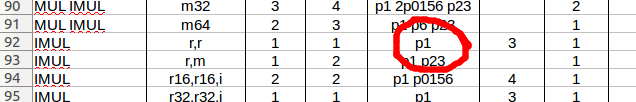
… or from uops.info:
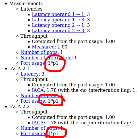
On modern Intel some simple integer arithmetic (add, sub, inc, dec), bitwise (or, and, xor) and test (test, cmp) run on four ports, so you aren’t very likely to see a port bottleneck for these operations (since the pipeline width bottleneck is more general and is also four), but many operations complete for only a few ports. For example, shift instructions and bit test/set operations like bt, btr and friends use only p1 and p6. More advanced bit operations like popcnt and tzcnt excecute only p1, and so on. Note that in some cases instructions which can go to wide variety of ports, such as add may execute on a port that is under contention by other instructions rather than on the less loaded ports: a scheduling quirk that can reduce performance. Why that happens is not fully understood.
One of the most common cases of port contention is with vector operations. There are only three vector ports, so the best case is three vector operations per cycle, and for AVX-512 there are only two ports so the best case is two per cycle. Furthermore, only a few operations can use all three ports (mostly simple integer arithmetic and bitwise operations and 32 and 64-bit immediate blends) – many are restricted to one or two ports. In particular, shuffles run only on p5 and can be a bottleneck for shuffle heavy algorithm.
Tools
In the example above it was easy to see the port pressure because the imul instructions go to only a single port, and the remainder of the instructions are mostly simple instructions that can go to any of four ports, so a 4 cycle solution to the port assignment problem is easy to find. In mode complex cases, with many instructions that go to many ports, it is less clear what the ideal solution is (and even less clear what the CPU will actually do without testing it), so you can use one of a few tools:
Intel IACA
Tries to solve for port pressure (algorithm unclear) and displays it in a table. Has reached end of life but can still be downloaded here.
RRZE-HPC OSACA
Essnentially an open-source version if IACA. Displays cumulative port pressure in a similar way to IACA, although it simply divides each instruction evenly among the ports it can use and doens’t look for a more ideal solution. On github.
LLVM-MCA
Another tool similar to IACA and OSACA, shows port pressure in a similar way and attempts to find an ideal solution (algorithm unclear, but it’s open source so someone could check). Comes with LLVM 7 or higher and documentation is here.
Measuring It
You can measure the actual port pressure using the perf and the uops_dispatched_port counters. For example, to measure the full port pressure across all 8 ports, you can do the following in uarch-bench:
./uarch-bench.sh --timer=perf --test-name=cpp/mul-4 --extra-events=uops_dispatched_port.port_0,uops_dispatched_port.port_1,uops_dispatched_port.port_2,uops_dispatched_port.port_3,uops_dispatched_port.port_4,uops_dispatched_port.port_5,uops_dispatched_port.port_6,uops_dispatched_port.port_7
...
Running benchmarks groups using timer perf

** Running group cpp : Tests written in C++ **
           Benchmark       Cycles       uops_d       uops_d       uops_d       uops_d       uops_d       uops_d       uops_d       uops_d
Four multiplications         4.00         1.06         4.00         0.50         0.50         0.00         0.97         1.81         0.00
While noting that that the column naming scheme is really bad in this case, we see that the port1 (the 3rd numeric column) has 4 operations dispatched every iteration, and iterations take 4 cycles, so the port is active every cycle, i.e., 100% pressure. None of the other ports have significant pressure at all, they are all active less than 50% of the time.
Remedies
- Of course, any solution that removes instructions causing port pressure can help, so most of the same remedies that apply to the pipeline width limit also apply here.
- Additionally, you might try replacing instructions which content for a high-pressure port with others that use different ports, even if the replacement results in more total instructions/uops. For example, sometimes p5 shuffle operations can be replaced with blend operations: you need more total blends but the resulting code can be faster since the blends execute on otherwise underused p0 and p1. Some 32 and 64-bit register-to-register broadcasts that use p5 don’t use p5 at all if you instead use a memory source, a rare case where memory source can be faster than register source for the same operation.
Load Throughput Limit
Intel, AMD: 2 loads per cycle
Modern Intel and AMD chips (and many others) have a limit of two loads per cycle, which you can achieve if both loads hit in L1. You could just consider this the same as the “port pressure” limit, since there only two load ports – but the limit is interested enough to call out on its own.
Of course, like all limits this is a best case scenario: you might achieve much less than two loads if you are not hitting in L1. Still, it is intersting to note how high this limit is: given the pipeline width of four, fully half of your instructions can be loads while still running at maximum speed.
It’s not all that common to this hit this limit, but you can certainly do it. The loads have to be mostly independent (not part of a carried dependency chain), since otherwise the load latency will limit you more than the throughput.
It’s not all that common to hit this limit, but it can often happen in an indirect load scenario (where part of the load address is itself calculated using a value from memory), or when heavy use of lookup tables is made. Consider the following loop, does an indirect loop in data based on the offsets array and sums the values it finds11:
do {
    sum1 += data[offsets[i - 1]];
    sum2 += data[offsets[i - 2]];
    i -= 2;
} while (i);
This compiles to the following assembly:
88:                                       ; total fused uops
    mov    r8d,DWORD PTR [rsi+rdx*4-0x4]  ; 1
    add    ecx,DWORD PTR [rdi+r8*4]       ; 2
    mov    r8d,DWORD PTR [rsi+rdx*4-0x8]  ; 3
    add    eax,DWORD PTR [rdi+r8*4]       ; 4
    sub    rdx,0x2                        ; (fuses w/ jne)
    jne    88                             ; 5
There are only 5 fused-uops12 here, so maybe this executes in 1.25 cycles? Not so fast – it takes 4 cycles because there are 4 loads and we have a speed limit of 2 loads per cycle13.
Note that gather instructions count “one” against this limit for each element they they load. vpgatherdd ymm0, ... for example, counts as 8 against this limit since it loads eight elements.
Split Cache Lines
For the purposes of this speed limit, all loads that hit in the L1 cache count as one, except loads that split a cache line. That is, loads of two bytes or more which cross a 64-byte boundary. Such loads count as two. If your loads are naturally aligned, you will never split a cache line. If your loads have totally random alignment, how often you split a cache line depends on the load size: for a load of N bytes, you’ll split a cache line with probability (N-1)/64. Hence, 32-bit random unaligned loads split less than 5% of the time but 256-bit AVX loads split 48% of the time and AVX-512 loads more than 98% of the time.
Remedies
If you are lucky enough to hit this limit, you just need less loads. Note that the limit is not expressed in terms of the number of bytes loaded, but in the number of separate loads. So sometimes you can combine two or more adjacent loads into a single load. An obvious application of that is vector loads: 32-byte AVX loads still have the same limit of two per cycle as byte loads. It is difficult to use vector loads in concert with scalar code however: although you can do 8x 32-bit loads at once, if you want to feed those loads to scalar code you have trouble, because you can’t efficiently get that data into scalar registers14. That is, you’ll have to work on vectorizing the code that consumes the loads as well.
You can also sometimes use wider scalar loads in this way. In the example above, we do four 32-bit loads – two of which are scattered (the access to data[]), but two of which are adjacent (the accesses to offsets[i - 1] and offsets[i - 2]). We could combine those two adjacent loads into one 64-bit load, like so15:
do {
    uint64_t twooffsets;
    std::memcpy(&twooffsets, offsets + i - 2, sizeof(uint64_t));
    sum1 += data[twooffsets >> 32];
    sum2 += data[twooffsets & 0xFFFFFFFF];
    i -= 2;
} while (i);
This compiles to:
98:                                        ; total fused uops
    mov    rcx,QWORD PTR [rsi+rdx*4-0x8]   ; 1
    mov    r9,rcx                          ; 2
    mov    ecx,ecx                         ; 3
    shr    r9,0x20                         ; 4
    add    eax,DWORD PTR [rdi+rcx*4]       ; 5
    add    r8d,DWORD PTR [rdi+r9*4]        ; 6
    sub    rdx,0x2                         ; (fuses w/ jne)
    jne    98                              ; 7
We have 7 fused-domain uops rather than 5, yet this runs in 1.81 cycles, about 10% faster. The theoretical limit based on pipeline width is 7 / 4 = 1.75 cycles, so we are proably getting collisions on p6 between the shr and the taken branch (unrolling a bit more would help). Clang 5.0 manages to do better, by one uop:
70:
    mov    r8,QWORD PTR [rsi+rdx*4-0x8]
    mov    r9d,r8d
    shr    r8,0x20
    add    ecx,DWORD PTR [rdi+r8*4]
    add    eax,DWORD PTR [rdi+r9*4]
    add    rdx,0xfffffffffffffffe
    jne    70
It avoided the mov r9,rcx instruction by combining that and the zero extension (which is effectively the & 0xFFFFFFFF) into a single mov r9d,rd8. It runs at 1.67 cycles per iteration, saving 20% over the 4-load version, but still slower than the 1.5 limit implied by the 4-wide fused-domain limit.
This code is an obvious candidate for vectorization with gather, which could in principle approach 1.25 cycles per itration (8 gathered loads + 1 256-bit load from offset per 4 iterations) and newer clang versions even manage to do it, if you allow some inlining so they can see the size and alignment of the buffer. However, the result is not good: it was more than twice as slow as the scalar approach.
Memory and Cache Bandwidth
The load and store limits discuss the ideal scenario where loads and stores hit in L1 (or hit in L1 “on average” enough to not slow things down), but there are throughput limits for other levels of the cache. If your know your loads hit primarily in a particular level of the cache you can use these limits to get a speed limit.
The limits are listed in cache lines per cycle and not in bytes, because that’s how you need to count the accesses: in unique cache lines accessed. The hardware transfers full lines. You can achieve these limits, but you may not be able to consume all the bytes from each cache line, because demand accesses to the L1 cache cannot occur on the same cycle that the L1 cache receives data from the outer cache levels. So, for example, the L2 can provide 64 bytes of data to the L1 cache per cycle, but you cannot also access 64 bytes every cycle since the L1 cannot satisfy those reads from the core and the incoming data from the L2 every cycle. All the gory details are over here.
| Microarchitecture | L2 | L3 |
| CNL | 0.75 | 0.2 – 0.3 |
| SKX | 1 | ~0.1 (?) |
| SKL | 1 | 0.2 – 0.3 |
| HSW | 0.5 | 0.2 – 0.3 |
The very poor figure of 0.1 cache lines per cycle (about 6-7 bytes a cycle) from L3 on SKX is at odds with Intel’s manuals, but it’s what I measured on a W-2104. For architectures earlier than Haswell I think the numbers will be similar back to Sandy Bridge.
If your accesses go to a mix of cache levels: you will probably get slightly worse bandwidth than what you’d get if you calculated the speed limit based on the assumption the cache levels can be accessed independently.
Memory bandwidth is a bit more complicated. You can calculate your theoretical value based on your memory channel count (or look it up on ARK), but this is complicated by the fact that many chips cannot reach the maximum bandwidth from a single core since they cannot generate enough requests to saturate the DRAM bus, due to limited fill buffers. So you are better off just measuring it.
Remedies
The usual remedies to improve caching performance apply: pack your structures more tightly, try to ensure locality of reference and prefetcher friendly access patterns, use cache blocking, etc.
Carried Dependency Chains
Sum of latencies in the longest carried dependency chain
Everything discussed so far is a limited based on throughput – the machine can only do so many things per cycle, and we count the number of things and apply those limits to determine the speed limit. We don’t care about how long each instruction takes to finish (as long as we can start one per cycle), or from where it gets its inputs. In practice, that can matter a lot.
Let’s consider, for exmaple, a modified version of the multiply loop above, one that’s a lot simpler:
for (size_t i = 0; i < len; i++) {
    uint32_t x = data[i];
    product *= x;
}
This does only a single multiplication per iteration, and compiles to the following tight loop:
50:
    imul   eax,DWORD PTR [rdi]
    add    rdi,0x4
    cmp    rdi,rdx
    jne    50
That’s only 3 fused uops, so our pipeline speed limit is 0.75 cycles/iteration. But wait, we know the imul needs p1, and the other two operations can go to other ports, so the p1 pressure means a limit of 1 cycle/iteration. What does the real world have to say?
./uarch-bench.sh --timer=perf --test-name=cpp/mul-chain --extra-events=$PE_PORTS
              Benchmark       Cycles       uops_d       uops_d       uops_d       uops_d       uops_d       uops_d       uops_d       uops_d
Chained multiplications         2.98         0.50         1.00         0.50         0.50         0.00         0.50         1.00         0.00
Bleh, 2.98 cycles, or 3x slower than we predicted.
What happened? As it turns out, the imul instruction has a latency of 3 cycles. That means that the result is not available until 3 cycles after the operation starts executing. This contrasts with 1 latency cycle for most simple arithmetic operations. Since on each iteration the multiply instruction depends on the result of the result of the previous iteration’s multiply16, every multiply can only start when the previous one finished, i.e., 3 cycles later. So 3 cycles is the speed limit for this loop.
Note that we mostly care about loop carried dependencies, which are dependency chains that cross loop iterations, i.e., where some output register in one iteration is used as an input register for the same chain in the next iteration. In the example, the carried chain involves only eax, but more complex chains are common in practice. In the earlier example, the four imul instructions did form a chain:
930:
    mov    r10d,DWORD [rdi+rcx*4+0x4] ; load
    mov    r8d,r10d                   ;
    imul   r8d,ecx                    ; imul1
    imul   r8d,edx                    ; imul2
    imul   r8d,ecx                    ; imul3
    add    rcx,0x1                    ;
    imul   r8d,r9d                    ; imul4
    mov    r9d,r10d                   ;
    add    eax,r8d                    ; add
    cmp    rcx,rsi                    ;
    jne    930                        ;
Note how each imul depends on the previous through the input/output r8d. Finally, the result is added to eax ,and eax is indeed used as input in the next iteration, so do we have a loop-carried dependency chain? Yes – but a very small one involving only eax. The dependency chain looks like this:
iteration 1       load -> imul1 -> imul -> imul -> imul -> add
                                                            |
                                                            v
iteration 2       load -> imul1 -> imul -> imul -> imul -> add
                                                            |
                                                            v
iteration 3       load -> imul1 -> imul -> imul -> imul -> add
                                                            |
                                                            v
etc ...                                                    ...
So yes, there is a dependent chain there, and the imul instructions are connected to that chain, but they don’t particpate in the carried part. Only the single-cycle latency add instruction participates in the carried dependency chain, so the implied speed limit is 1 cycle/iteration. In fact, all of our examples so far have had carried dependency chains, but they have all been small enough never to be the dominating factor. You may also have multiple carried dependency chains in a loop: the speed limit is set by the longest.
I’ve only touched on this topic and won’t go much further here: for a deeper look check out Fabian Giesen’s A whirlwind introduction to dataflow graphs.
Finally, you may have noticed something interesting about the benchmark result of 2.98 cycles. In every other case, the measured time was equal or slightly more than the speed limit, due to test overhead. How were we able to break the speed limit in this case and come under 3.00 cycles, albeit by less than 1%? Maybe it’s just measurement error – the clocks aren’t precise enough time this more precisely?
Nope. The effect is real and is due to the structure of the test. We run the multiplication code shown above on a buffer of 4096 elements, so the there are 4096 iterations. The benchmark loop that calls that function, itself runs 1000 iterations, each one calling the 4096-iteration inner loop. What happens to get the 2.98 is that in between each call of the inner loop, the multiplication chains can be overlapped. Each chain is 4096-elements long, but the start each function starts a new chain:
uint32_t mul_chain(const uint32_t *data, size_t len, uint32_t m) {
    uint32_t product = 1;
    for (size_t i = 0; i < len; i++) {
      // ...
Note the product = 1 – that’s a new chain. So some small amount of overlap is possible near the end of each loop, which shaves about 80-90 cycles off the loop time (i.e., somethign like ~30 multiplications get to overlap). The size of the overlap is limited by the out-of-order buffer structures in the CPU, in particular the re-order buffer and scheduler.
Tools
As fun as tracing out dependency chains by hand is, you’ll eventually want a tool to do this for you. All of IACA, OSACA and llvm-mca can do this type of latency analysis and identity loop carried dependencies implicity. For example, llvm-mca correctly identifies that this loop will take 3 cycles/iteration.
Remedies
The basic remedy is that you have to shorten or break up the dependency chains.
For example, maybe you can use lower latency instructions like addition or shift instead of multiplication. A more generally applicable trick is to turn one long dependency chain into several parallel ones. In the example above, the associativity property of integer multiplication17 allows us to do the multiplications in any order. In particular, we could accumulate every third element into a separate product and multiply them all at the end, like so:
    uint32_t p1 = 1, p2 = 1, p3 = 1, p4 = 1;
    for (size_t i = 0; i < len; i += 4) {
        p1 *= data[i + 0];
        p2 *= data[i + 1];
        p3 *= data[i + 2];
        p4 *= data[i + 3];
    }
    uint32_t product = p1 * p2 * p3 * p4;
This test runs at 1.00 cycles per iteration, so the latency chain speed limit has been removed. Well, it’s still there: each iteration above takes at least 3 cycles because of the four carried dependency chains between each iteration, but since we are doing 4x as much work now, the p1 port limit becomes the dominant limit.
Compilers can sometimes make this transformation for you, but not always. In particular, gcc is reluctant to unroll loops at any optimization level, and unrolling loops is often a prerequisite for this transformation, so often you are stuck doing it by hand.
Front End Effects
I’m going to largely gloss over this one. It really deserves a whole blog post, but in recent Intel and AMD architecturs the prevalence of front-end effects being the limiting factor in loops has dropped a lot. The introduction of the uop cache and better decoders means that it is not as common as it used to be. For a complete18 treatment see Agner’s microarchitecture guide, starting with section 9.1 through 9.7 for Sandy Bridge (and then the corresponding sections for each later uarch you are interested in).
If you see an effect that depends on code alignment, especially in a cyclic pattern with a period 16, 32 or 64 bytes, it is very likely to be a front-end effect. There are hacks you can use to test this.
First are simple absolute front-end limits to delivered uops/cycle depeneding on where the uops are coming from19:
Table 1: Uops delivered per cycle
| Architecture | Microcode (MSROM) | Decoder (MITE) | Uop cache (DSB) |
|---|---|---|---|
| <= Broadwell | 4 | 4 | 4 |
| >= Skylake | 4 | 5 | 6 |
These might look like important values. I even made a table, one of only two in this whole post. They aren’t very important though, because they are all equal to or larger than the pipeline limit of 4. In fact it is hard to even carefully design a microbenchmark which definitively shows the difference between the 5-wide decode on SKL and the 4-wide on Haswell and earlier. So you can mostly ignore these numbers.
The more important limitations are specific to the individual sources. For example:
- The legacy decoder (MITE) can only handle up to 16 instruction bytes per cycle, so any time instruction length averages more than four bytes decode throughput will necessarily be lower than four. Certain patterns will have worse throughput than predicted by this formula, e.g., 7 instructions in a 16 byte block will decode in a 6-1-6-1 pattern.
- Only one of the 4 or 5 legacy decoders can handle instructions which generate more than one uop, so a series of instructions which generate 2 uops will only decode at 1 per cycle (2 uops per cycle).
- Only one uop cache entry (with up to 6 uops) can be accessed per cycle. For larger loops this rarely a bottleneck, but it means that any loop that crosses a uop cache boundary (32 bytes up to and including Broadwell, 64 bytes in Skylake and beyond) will always take 2 cycles, since two uop cache entries are involved. It is not unusual to find small loops which normally take as little as 1 cycle split by such boundaries suddenly taking 2 cycles.
- Instructions which use microcode, such as gather (pre-Skylake) have additional restrictions and throughput limitations.
- The LSD suffers from reduced throughput at the boundary between one iteration and the next, although hardware unrolling reduces the impact of the effect. Full details are on StackOveflow. Note that the LSD is disabled on most recent CPUs due to a bug. It is re-enabled on some of the most recent chips (CNL and maybe Cascade Lake).
Again, this is only scratching the surface – see Agner for a comprehensive treatment.
Stores
1 store per cycle
Modern Intel and AMD CPUs can perform at most one store per cycle. No matter what, you won’t exceed that. For many algorithms that make a predictable number of stores, this is a useful upper bound on a performance. For example, a 32-bit radix sort that makes 4 passes and does a store per element for each pass will never operate faster than 4 cycles per element (in radix sort, actual performance usually ends up much worse so this isn’t the dominant factor for most implementations).
This limit applies also to vector scatter instructions, where each element counts as “one” against this limit. Like loads, a store that crosses a cache line counts as two, but other unaligned stores only count as on Intel. On AMD the situation is more complicated: the penalties for stores that cross a boundary is larger, and it’s not just 64-byte boundaries that matter – more details here.
Remedies
Remove unecessary stores from your core loops. If you are often storing the same value repeatedly to the same location, it can even be profitable to check that the value is differnet, which requires a load, and only do the store if different, since this can replace a store with a load. Most of all, you want to take advantage of vectorized stores if possible: you can do 8x 32-bit stores in one cycle with a single vectorized store. Of course, if your stores are not contiguous, this will be difficult or impossible.
Complex Addressing Limit
Max of 1 load (any addressing) concurrent with a store with complex addressing per cycle.
This limit is Intel specific.
The load and store limits above are written as if they are independnet. That is, they imply that you can do 2 loads and 1 store per cycle. Sometimes that is true, but it depends on the addressing modes used.
Each load and store operation needs an address generation which happens in an AGU. There are three AGUs on modern Intel chips: p2, p3 and p7. However, p7 is restricted: it can only be used by stores, and it can only be used if the store addressing mode is simple. Simple addressing is anything that is of the form [base_reg + offset] where offset is in [0, 2047]. So [rax + 1024] is simple addressing, but all of [rax + 4096], [rax + rcx * 2] and [rax * 2] are not.
To apply this limit, count all load and any stores with complex adressing: these operations cannot execute at more than 2 per cycle.
Remedies
At the assembly level, the main remedy is make sure that your stores use simple addressing modes. Usually you do this by incrementing a pointer by the size of the element rather indexed addressing modes.
That is, rather than this:
mov [rdi + rax*4], rdx
add rax, 1
You want this:
mov [rdi], rdx
add rdi, 4
Of course, that’s often simpler said than done: indexed addressing modes are very useful for using a single loop counter to access multiple arrays, and also when the value of the loop counter is directly used in the loop (as opposed to simply being used for addressing). For example, consider the following loop which writes the element-wise sum of two arrays to a third array:
void sum(const int *a, const int *b, int *d, size_t len) {
    for (size_t i = 0; i < len; i++) {
        d[i] = a[i] + b[i];
    }
}
The loop compiles to the following assembly:
.L3:
    mov     r8d, DWORD PTR [rsi+rax*4]
    add     r8d, DWORD PTR [rdi+rax*4]
    mov     DWORD PTR [rdx+rax*4], r8d
    add     rax, 1
    cmp     rcx, rax
    jne     .L3
This loop will be limited by the complex adressing limitation to 1.5 cycles per iteration, since there are 1 store that uses complex addressing, plus one load.
We could use separate pointers for each array and increment all of them, like:
.L3:
    mov     r8d, DWORD PTR [rsi]
    add     r8d, DWORD PTR [rdi]
    mov     DWORD PTR [rdx], r8d
    add     rsi, 4
    add     rdi, 4
    add     rdx, 4
    cmp     rcx, rdx
    jne     .L3
Everything uses simple addressing, great! However, we’ve added two uops and so the speed limit is pipeline width: 7/4 = 1.75, so it will probably be slower than before.
The trick is to only use simple addressing for the store, and calculate the load addresses relative to the store address:
.L3:
    mov     eax, DWORD PTR [rdx+rsi] ; rsi and rdi have been adjusted so that
    add     eax, DWORD PTR [rdx+rdi] ; rsi+rdx points to a and rdi+rdx to b
    mov     DWORD PTR [rdx], eax
    add     rdx, 4
    cmp     rcx, rdx
    ja      .L3
When working in a higher level language, you may not always be able to convince the compiler to generate the code we want as it might simply see through our transfomations. In this case, however, we can convince gcc to generate the code we want by writing out the transformation outselves:
void sum2(const int *a, const int *b, int *d, size_t len) {
    int *end = d + len;
    ptrdiff_t a_offset = (a - d);
    ptrdiff_t b_offset = (b - d);
    for (; d < end; d++) {
        *d = *(d + a_offset) + *(d + b_offset);
    }
}
This is UB all over the place if you pass in arbitrary arrays, because we subtract unrelated pointers (a - d) and use pointer arithmetic which outside of the bounds of the original array (d + a_offset) – but I’m not aware of any compiler that will take advantage of this (as a standalone function it seems unlikely that will ever be the case: because the arrays all could be related, so the function isn’t always UB). Still you should avoid stuff like this unless you have a really good reason to push the boundaries. You could achieve the same effect with uintptr_t which isn’t UB but only unspecified, and that will work on every platform I’m aware of.
Another way to get simple addressing without adding too much overhead for separate loop pointers is to unroll the loop a little bit. The increment only needs to be done once per iteration, so every unroll reduces the cost.
Note that even if stores have non-complex addressing, it may not be possible to sustain 2 loads/1 store, because the store may sometimes choose one of the port 2 or port 3 AGUs instead, starving a load that cycle.
Taken Branches
Intel: 1 per 2 cycles (see exception below)
If you believe the instruction tables, one taken branch can be taken per cycle, but experiments show that this is true only for very small loops with a single backwards branch. For larger loops or any forward branches, the limit is 1 per 2 cycles.
So avoid many dense taken branches: organize the likely path instead as untaken. This is something you want to do anyways for front-end throughput and code density.
Out of Order Limits
Here we will cover several limits which all effect the effective window over which the processor can reorder instructions. It is not a hard limit in itself: you can’t use it to directly establish an upper bound on cycles per iterations or whatever (i.e., the units for these values aren’t “per cycle”) – but you can use it in concert with other analysis to refine the estimate.
Until now, we have been implicitly assuming an infinite out of order window. That’s why we said, for example, that only loop carried dependencies matter when calculating dependency chains; the implicit assumption is that there is enough out-of-order magic to reorder different loop iterations to hide the effect of all the other chains. Of course, on real CPUs, there is a limit to the magic: if your loops have 1,000 instructions per iteration, the will CPU will not be able to overlap the much of each iteration at all: the different iterations are too far apart in instruction stream for significant overlap.
All the discussion here refers to the dynamic instruction stream – which is the actual stream of instructions seen by the CPU. This is opposed to the static instruction stream, which is the series of instructions as they appear in the binary. Inside a basic block, static and dynamic instruction streams are the same: the difference is that the dynamic stream follows all jumps, so it is a trace of actual execution.
For example, take the following nested loops, with inner and outer iteration counts of 2 and 4:
    xor rdx, rdx
    mov rax, 2

outer:
    mov rcx, 4

inner:
    add rdx, rcx
    dec rcx
    jnz inner

    dec rax
    jnz outer
The static instruction stream is just want you see above, 8 instructoins in total. The dynamic instructon stream traces what happens at runtime, so the inner loop appears 8 times, for example:
    xor rdx, rdx
    mov rax, 2

    ; first iteration of outer loop
    mov rcx, 4

    ; inner loop 4x
    add rdx, rcx
    dec rcx
    jnz inner

    add rdx, rcx
    dec rcx
    jnz inner

    add rdx, rcx
    dec rcx
    jnz inner

    add rdx, rcx
    dec rcx
    jnz inner

    jnz outer

    ; second iteration of outer loop
    mov rcx, 4

    ; inner loop 4x
    add rdx, rcx
    dec rcx
    jnz inner

    add rdx, rcx
    dec rcx
    jnz inner

    add rdx, rcx
    dec rcx
    jnz inner

    add rdx, rcx
    dec rcx
    jnz inner

    jnz outer

    ; done!
All that to say that when you are thinking about out of order window, you have to think about the dynamic instruction/uop stream, not the static one. For a loop body with no jumps or calls, you can ignore this distinction.
With that background out of the way, let’s look at the various OoO limits next. Most of these limits have the same effect which is to limit the available out-of-order window, stalling issue until a resource becomes available. They differ mostly in what they count, and how many of that thing can be buffered.
Reorder Buffer Size
Intel SNB: 168 fused uops
Intel IVB: 168 fused uops
Intel HSW: 192 fused uops
Intel BDW: 192 fused uops
Intel SKL: 224 fused uops (including SKX)
Intel SNC: 352 (reported)
AMD Zen: 192 mops
AMD Zen2: 224 mops
The reorder buffer holds instructions from the point at which they are allocated (issued, in Intel speak) until they retire. It puts a hard upper limit on the OoO window as measured from the oldest unretired instruction to the newest instruction that be issued.
As an example, a load instruction takes a cache miss which means it cannot retire until the miss is complete. On an Haswell machine with a ROB size of 192, at most 191 additional instructions can execute while waiting for the load: at that point the ROB window is exhausted and the core stalls. This puts an upper bound on the maximum IPC of the region of 192 / 300 = 0.64. It also puts a bound on the maximum MLP achievable, since only loads that appear in the next 191 instructions can (potentially) execute in parallel with the original miss. In fact, this behavior is used by Henry Wong’s robsize tool to measure the ROB size and other OoO buffer sizes, using a missed load followed by a series of filler instructions and finally another load miss. My varying the number of filler instructions and checking whether the loads executed in parallel or serially, the ROB size can be determined experimentally.
Remedies
If you are hitting the ROB size limit, you should switch from optimizing the code for the usual metrics and instead try to reduce the number of uops. For example, a slower (longer latency, less throughput) instruction can be used to replace two instructions which would otherwise be faster. Similarly, micro-fusion helps because the ROB limit counts in the fused domain.
Reorganizing the instruction stream can help too: if you hit the ROB limit after a specific long-latency instruction (usually a load miss) you may want to move expensive instructions into the shadow of that instruction so they can execute while the long latency instruction executes. In this way, there will be less work to do when the instruction completes. Similarly, you may want to “jam” loads that miss together: rather than spreading them out where they would naturally occur, putting them close together allows more of the to fit in the ROB window.
In the specific case of load misses, software prefetching can help a lot: it enables you to start a load early, but prefetches can retire before the load completes, so there is no stalling. For example, if you issue the prefetch 200 instructions before the demand load instruction, you have essentially broaded the ROB by 200 instructions as it applies to that load.
Register File Size Limit
Intel SNB: 160 integer, 144 vector
Intel IVB: 160 integer, 144 vector
Intel HSW: 168 integer, 168 vector
Intel SKL: 180 integer, 168 vector
AMD Zen: 168 integer, 160 vector
AMD Zen2: 180 integer, 160 vector
Every instruction with a destination register requires a renamed physical register, which is only reclaimed when the instruction is retired. These registers come from the physical regsiter file (PRF). So to fill the entire ROB with operations that require a destination register, you’ll need a PRF as large as the ROB. In practice, there are two separate register files on Intel and AMD chips: the integer registers file used for scalar registers such as rax and the vector register file used for SIMD registers such as xmm0, ymm0 and zmm0, and the sizes of these register files as shown above are somewhat smaller than the ROB size.
Not all of the registers are actually available for renaming: some are used to store the non-speculative values of the architectural registers, or for other purposes, so the available number of register is about 16 to 32 less than the values shown above. Henry Wong has a great description of observed available registers on the article I linked earlier, including some non-ideal behaviors that I’ve glossed over here. You can calculate the number of available registers on new architectures using the robsize tool.
The upshot is that for given ROB sizes, there are only enough registers available in each file for about 75% of the entries.
In practice, some instructions such as branches, zeroing idioms20 don’t consume PRF entries, which limit you hit depends on that ratio. Since integer and FP PRFs are distinct on recent Intel, you can consume from each PRF independently: meaning that vectorized code mixed with at least some GP code is unlikely to hit the PRF limit before it hits the ROB limit.
The effect of hitting the PRF limit is the same as the ROB size limit.
Remedies
There’s not all much you can do for this one beyond the stuff discussed in the ROB limit entry section. Maybe try to mix integer and vector code so you consume from each register file. Make sure you are using zeroing idioms like xor eax,eax rather than mov eax, 0 but you should already be doing that.
Branches in Flight
Intel: Maximum of 48 branches in flight
Modern Intel chips seem to have a limit of branches in flight, where in flight refers to branches that have not yet retired, usually because some older operation hasn’t yet completed. I first saw this limit described and measured here, although it seems like David Kanter had the scoop way back in 2012:
The branch order buffer, which is used to rollback to known good architectural state in the case of a misprediction is still 48 entries, as with Sandy Bridge.
The effects of exceeding the branch order buffer limit are the same as for the ROB limit.
Branches here refers to both conditional jumps (jcc where cc is some conditioanl code) and indirect jumps (things like jmp [rax]).
Remedies
Although you will rarely hit this limit, the solution is fewer branches. Try to move unecessary checks out of the hot path, or combine several checks into one. Try to organize multi-predictate conditions such that you can short-circuit the evaluation after the first check (so the subsequet checks don’t appear in the dynamic instruction stream). Consider replacing N 2-way (true/false) conditional jumps with one indirect jump with N^2 targets as this counts as only “one” instead of N against the branch limit. Consider conditional moves or other branch-free techniques.
Ensure that branches can retire as soon as possible, although in practice there often isn’t much opportunity to do this when dealing with already well-compiled code.
Note that many of these are the same things you might consider to reduce branch mispredictions, although they apply here even if there are no mispredictions.
Calls in Flight
Intel: 14-15
Only 14-15 to calls can be in-flight at once, exactly analagous to the limtiation on in-flight branches described above, except it applies to the call instruction rather than branches. As with the branches in-flight restriction, this comes from testing by Henry Wong, and in this case I am not aware of an earlier source.
Remedies
Reduce the number of call instructions you make. Consider ensuring the calls can be inlined, or partial inlining (a fast path that can be inlined combined with a slow path that isn’t). In extreme cases you might want to replace call + ret pairs with uncontional jmp, saving the return address in a register, plus indirect branch to return to the saved address. I.e. replace the following:
callee:
    ; function code goes here
    ret

; caller code
    call callee
With the following (which is essentially emulating the JAL instruction:
callee:
  ; function code goes here
  jmp [r15] ; return to address stashed in r15

; caller code
    movabs r15, next
    jmp callee
next:
This pattern is hard to achieve in practice in a high level language, although you might have luck emulating it with gcc’s labels as values functionality.
Bye
That’s it for now, if you made it this far I hope you found it useful.
Thanks to RWT forums users Paul A. Clayton, Adrian and Peter E. Fry, and HN users nkurz, maztheman and hyperpape for corrections and suggestions.
Thanks to Daniel Lemire for providing access to hardware on which I was able to test and verify some of these limits.
I don’t have a comments system yet, so I’m basically just outsourcing discussion to HackerNews right now: here is the thread for this post.